
Since the Kunming-Montreal Global Biodiversity Framework was adopted in 2022, “maintaining and restoring genetic diversity” in wild species is on the global agenda. The headline indicator A.4 – which all countries must report on from this year – is a simple measure of progress towards this goal. It estimates “the proportion of populations within species with an effective population size (Ne) > 500″. Today’s post zooms in on the effective population size – so, read on if you are curious why larger populations maintain more genetic diversity or if you’ve stumbled over the word “effective”!
What is genetic diversity?
Genetic diversity measures how many different versions of each gene exist in the population and how common they are (their frequencies). If you imagine each gene version as a different colour, as we do below, a more diverse population is a more colourful population. The more diversity there is, the more genetically different individuals are. For example, if there is only one version of a gene (low diversity – one colour, let’s say blue), all individuals are necessarily the same. But if there is a range of versions (colours), most individuals are different from each other.
Why does this matter? With more diversity, the population has better chances of having gene versions that match the environment when it changes – whether that’s because of human actions (like climate change) or natural events (like new diseases). More information about genetic diversity can be found here.
What does genetic diversity have to do with population size?
The number and frequency of gene versions in a population change over time because by chance, some individuals reproduce more than others. Let’s first look at this random process in a tiny population of only ten gene copies (points in the figure below). Ten gene copies correspond to five individuals, as each individual has two copies (top panel) – but it is easier to just think in terms of gene copies. For the gene we’re looking at, there are five different versions, shown in different colours, each starting out with two copies in the first generation (bottom panel; left). The next generation is produced through random reproduction of the 10 copies – some copies will have one or more “offspring” and others will have none, as indicated by the grey lines from generation 1 to generation 2. For example, the top orange copy in generation 1 has two offspring and the second orange copy has none. This process repeats each generation. Because there are so few copies, each one makes up a large share of the population: If one copy reproduces a lot, or not at all, that can strongly change version frequencies. For example, the purple version almost immediately disappears, just because two purple copies failed to reproduce. As a result, gene version frequencies change rapidly and most versions are lost quickly.
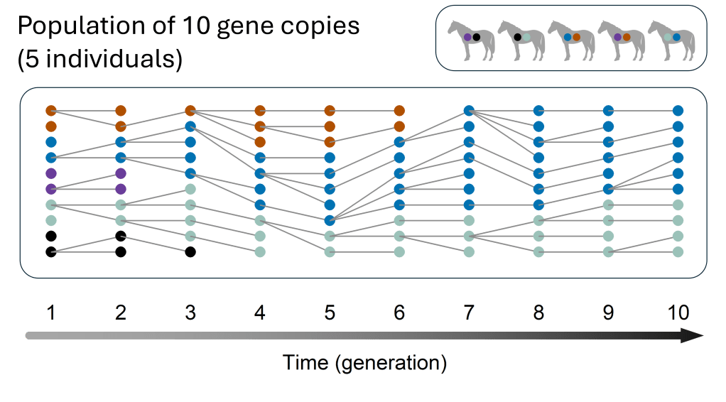
Example of a population of 10 gene copies. Each gene copy is represented by a point, and different colours represent different versions of the gene. The top panel shows that 10 gene copies correspond to 5 individuals (in this example, horses), as each individual carries two gene copies. The bottom panel shows how version frequencies randomly change over time. The versions are sorted by colour for visibility, but they are randomly distributed among individuals in the population. In the first generation (left), all versions have the same frequency (2/10=0.2). Copies reproduce randomly from generation to generation. “Parent copies” are connected to their “offspring copies” in the next generation by lines.
These random gene version frequency changes are called genetic drift. As we have seen, genetic drift is very pronounced in small populations. Let’s look at a larger population (50 copies) for comparison:
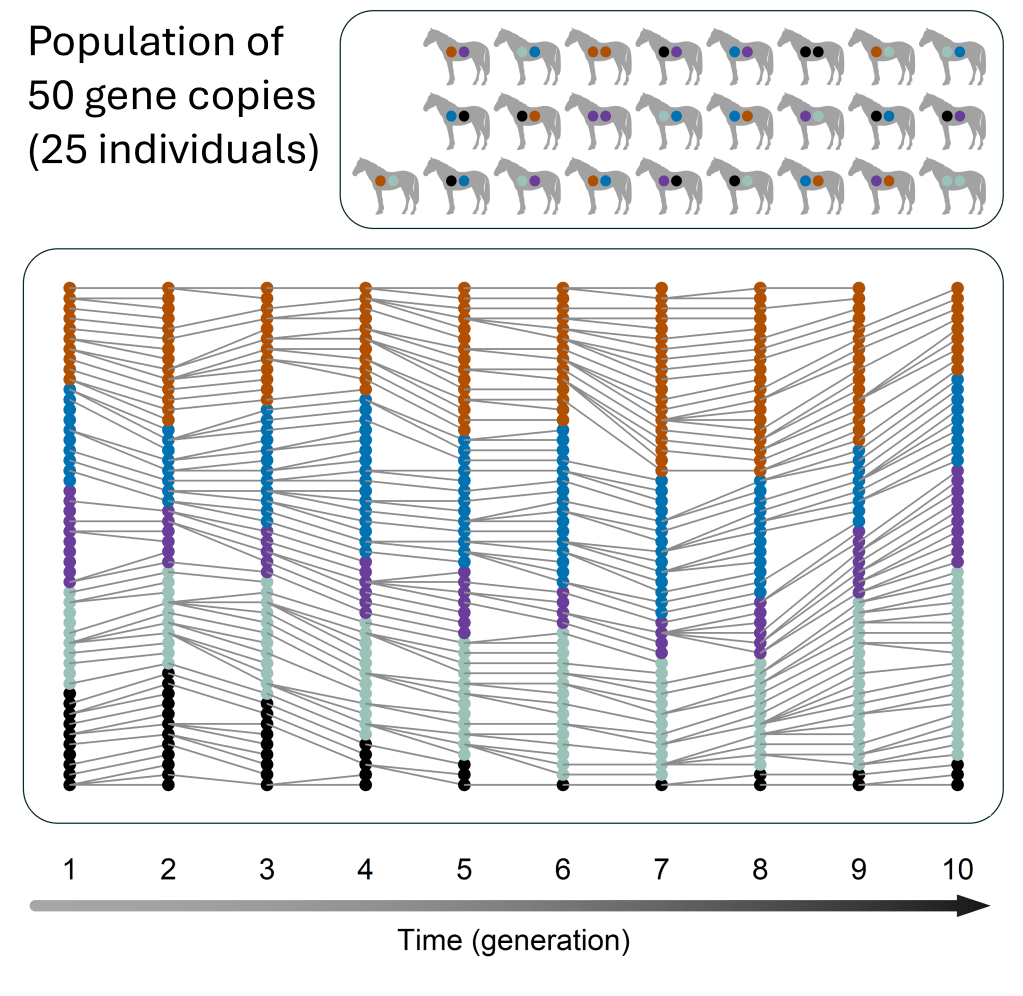
Example of a population of 50 gene copies.
Here, reproduction happens in the same random way as in the small population, and again each version starts out with the same frequency as in the figure above (a frequency of 0.2) – but in this larger population, individual chance events have a smaller effect because there are more copies in total. For example, there are again some purple copies that don’t reproduce, but purple isn’t lost completely because there are more purple copies in total. Purple copies that don’t reproduce can be balanced out by other purple copies that have more than one offspring. Gene version frequencies obviously still change over time, but these changes are less pronounced compared to the smaller population, and none of the gene versions are lost.
So, all else being equal, small populations lose genetic diversity more quickly over time and therefore tend to have lower genetic diversity. Importantly, this stronger influence of chance in small populations also affects beneficial gene versions – those that improve survival or reproduction. Even these beneficial gene versions can be lost by chance more easily when fewer copies are present.
Why we want to know the effective population size
So, it makes perfect sense that the headline genetic indicator is based on a measure of population size. However, there is a caveat – populations of the same censussize (Nc, the number of mature individuals) can lose genetic diversity at very different rates. For example, consider a population of Nc 1,000 where most individuals reproduce, versus one of the same size where far fewer do. Even if the total number of offspring is the same, the latter population loses genetic diversity faster: most offspring come from the same few parents. In terms of the figures above, this corresponds to a few gene copies having lots of offspring, while most gene copies have none at all – leading to dramatic random colour changes over time.
A classic example is the elephant seal, where very few dominant males mate with most of the females, and all the remaining males do not contribute to the next generation. Similarly, a population of Nc 1,000 in summer that drops to a much smaller size in winter (seasonal fluctuations, as common in many insects) will lose diversity faster than a stable population of 1,000 individuals.
This is where the effective population size, Ne, comes into play: It is a measure of population size that takes into account the extent of genetic drift – the more drift, the smaller Ne. In our example above, the first population of 1,000 individuals (where many individuals reproduce) will have a much larger Ne than the second population of 1,000 individuals (where only few individuals reproduce).
What is Ne? Click here for the short answer (without unicorns)
Ne is a measure of population size that doesn’t directly count the number of individuals, but instead reflects how many individuals actually pass on genes to the next generation and how similar their contributions are. The more individuals reproduce and the more similar their offspring numbers are, the larger is Ne. And the larger Ne, the less genetic diversity is lost over time. This plot shows that genetic diversity is lost much faster in a population with Ne 60 than one with Ne 600.
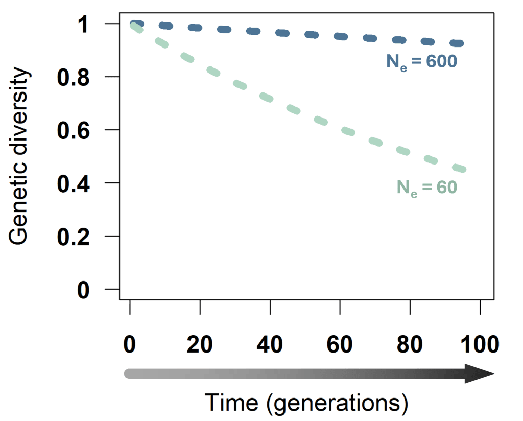
Genetic diversity (heterozygosity) loss over time in a population of Ne 600 (blue) and one of Ne 60 (turquoise).
What, exactly, is Ne? Click here for the long answer (with unicorns)
Ne is defined as the size of an idealised population that loses genetic diversity at the same rate as the population we’re interested in. An “idealised” population is an imaginary population without factors that increase genetic drift – for example, it is stable over time and all individuals produce a similar number of offspring. In the figure below, an idealised population of 600 individuals is shown in blue. It loses genetic diversity only very slowly. A real population of 600 individuals loses diversity much faster – for example, because few males contribute to the next generation (dark brown line). To determine Ne for the real population, we ask, How small must the idealised population be to lose diversity at the same rate as the real one? Here, Ne is 60: The diversity loss curve for an idealised population of 60 (turquoise) exactly coincides with that of the real population.
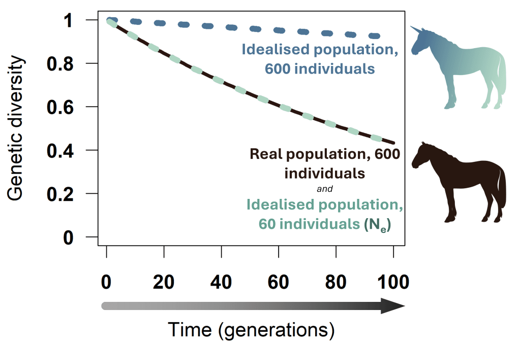
Genetic diversity (heterozygosity) loss over time in an example real population of size 600 individuals (brown) and idealised populations of 600 (blue) and 60 individuals (turquoise). The idealised population is symbolized by a unicorn, as it does not exist (we in GINAMO do not believe in unicorns), while the real population is symbolized by a horse. Studies have shown that Ne is much smaller than the count of mature individuals in both wild and domestic horse populations.
Ne is usually smaller than Nc
Ne is almost always smaller than Nc because many different factors in nature increase drift (Waples 2024). Ne/Nc ratios compiled from a range of different species can be found in the Supplementary Information of Hoban et al. 2020.
This work suggests that in many species, the Ne/Ncratio is around 0.1 or a bit larger (Hoban et al. 2020). However, the ratio does vary among species, and some species groups systematically deviate from this rule of thumb (the ratio is a bit higher in birds, for example). This is not surprising, given differences in life history traits such as reproductive strategies, life cycles, and other factors affecting Ne. For example, some birds lay only a few eggs per year and invest a lot in each, while many fish produce huge numbers of offspring, most of which die young. In the fish, parents can contribute much more unequally to the next generation, increasing drift and reducing Ne.
In our next blog post, we’ll discuss at what point Ne becomes too small – and how Ne, despite being a theoretical concept, can actually be estimated and used in practice!
